Introduction
Welcome to the project on Landslide Susceptibility Mapping and Exposure Assessment, part of the Master of Science in Geoinformatics at Politecnico di Milano. This project focuses on assessing and visualizing the risk of landslides in a specific region using a combination of advanced geospatial technologies and data analysis techniques.
What is a Landslide?
A landslide is the movement of rock, earth, or debris down a slope due to gravity. Landslides can be triggered by various factors including heavy rainfall, earthquakes, volcanic activity, or human activities such as construction. They pose significant risks to life, property, and the environment, making it crucial to identify and monitor susceptible areas.
Role of GIS and Remote Sensing
Geographic Information Systems (GIS) and remote sensing technologies are essential tools in landslide susceptibility mapping. GIS allows for the integration, analysis, and visualization of various geospatial data layers, helping to identify patterns and relationships. Remote sensing involves the acquisition of information about the Earth's surface from satellite or aerial sensors, providing critical data for monitoring and analysis.

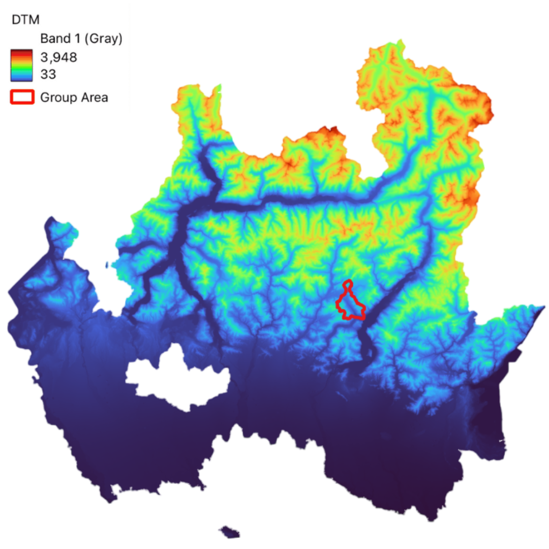
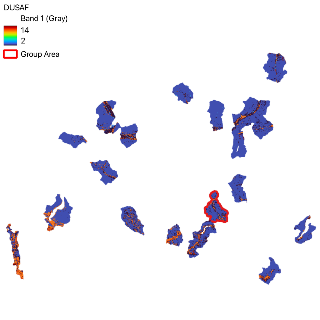
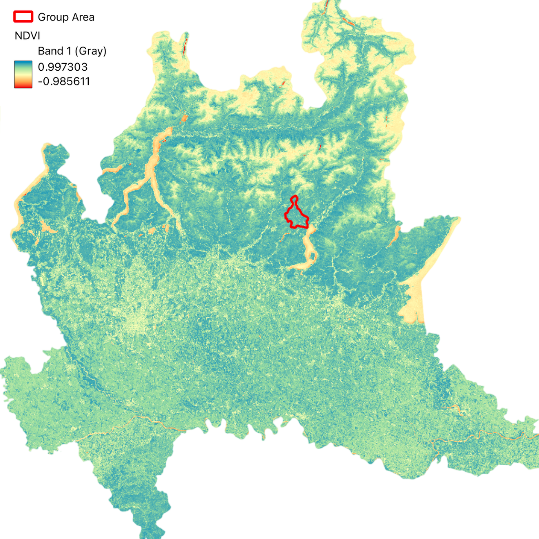
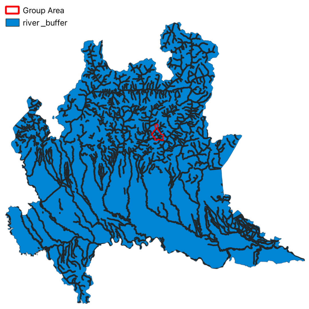
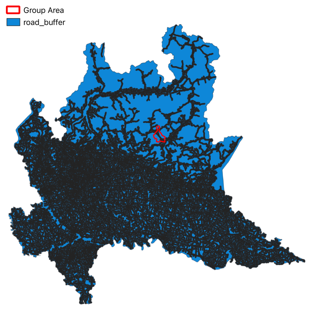
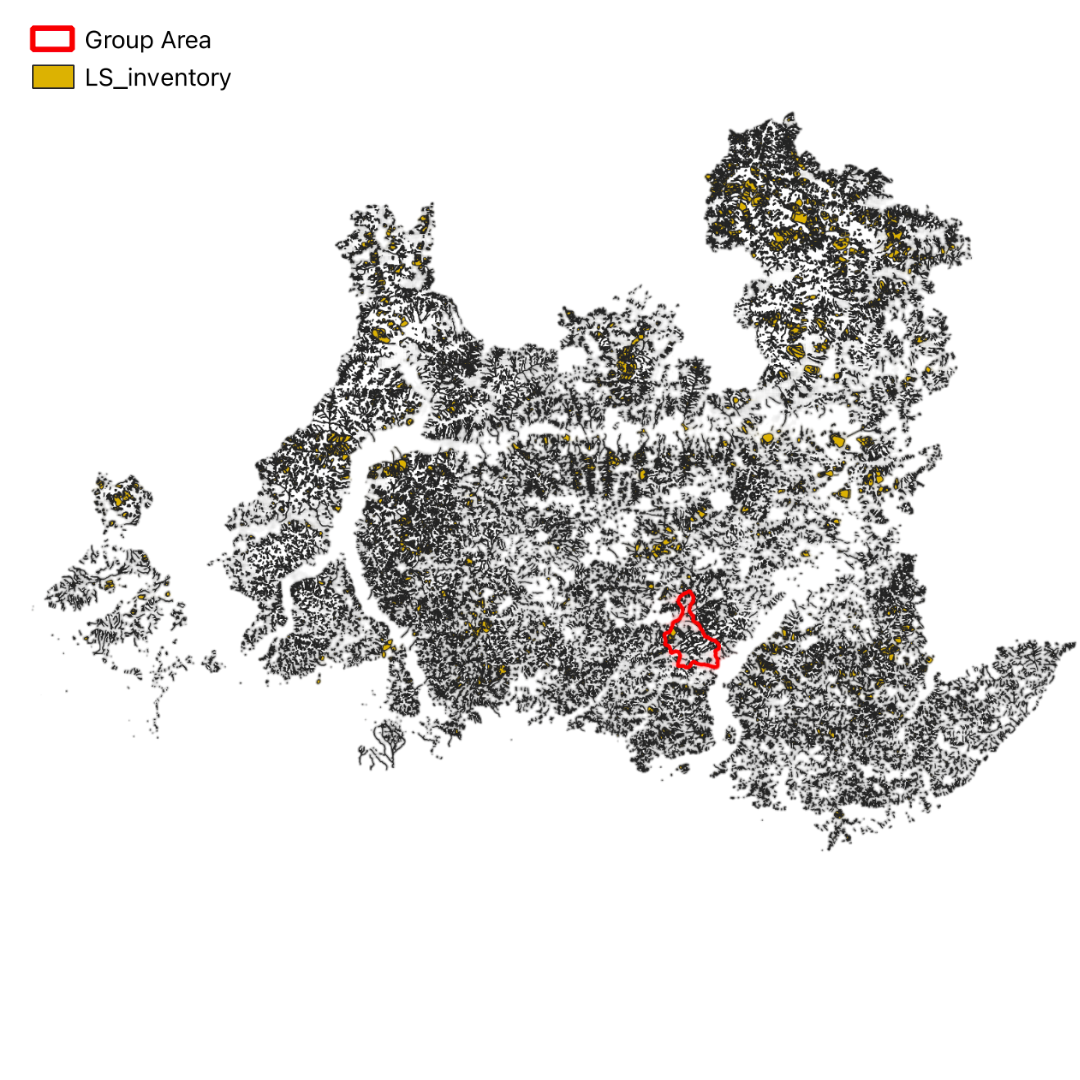
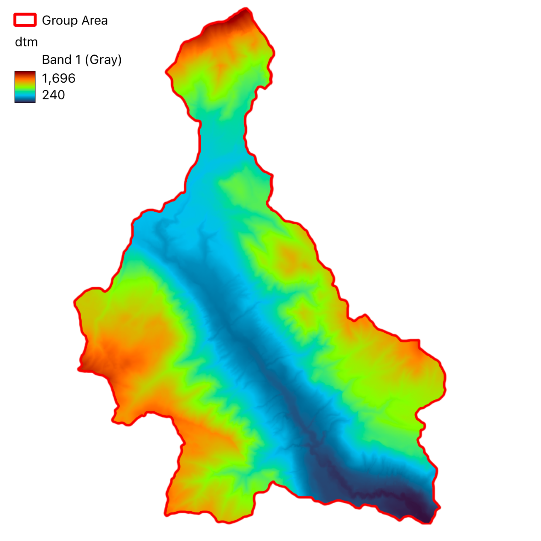
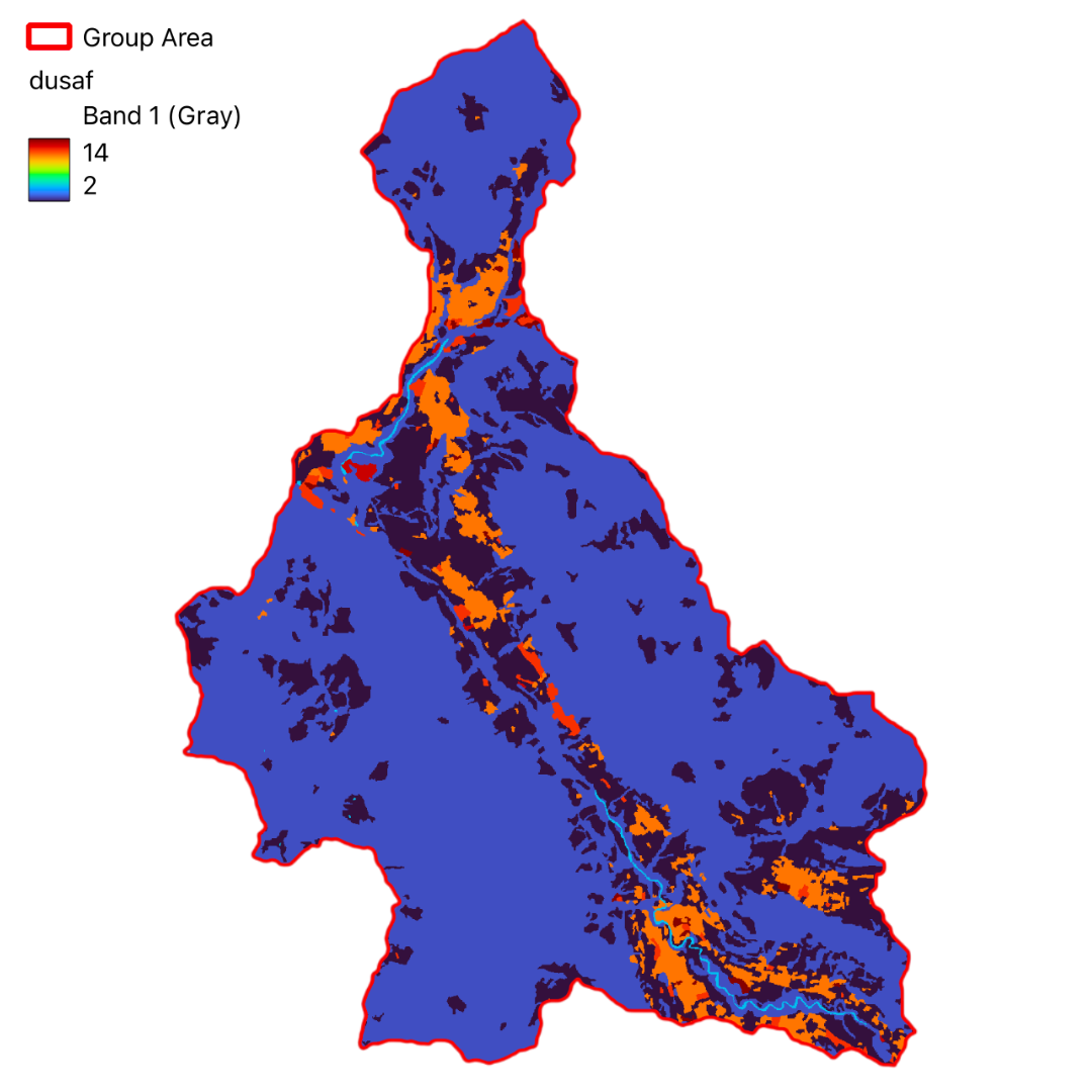
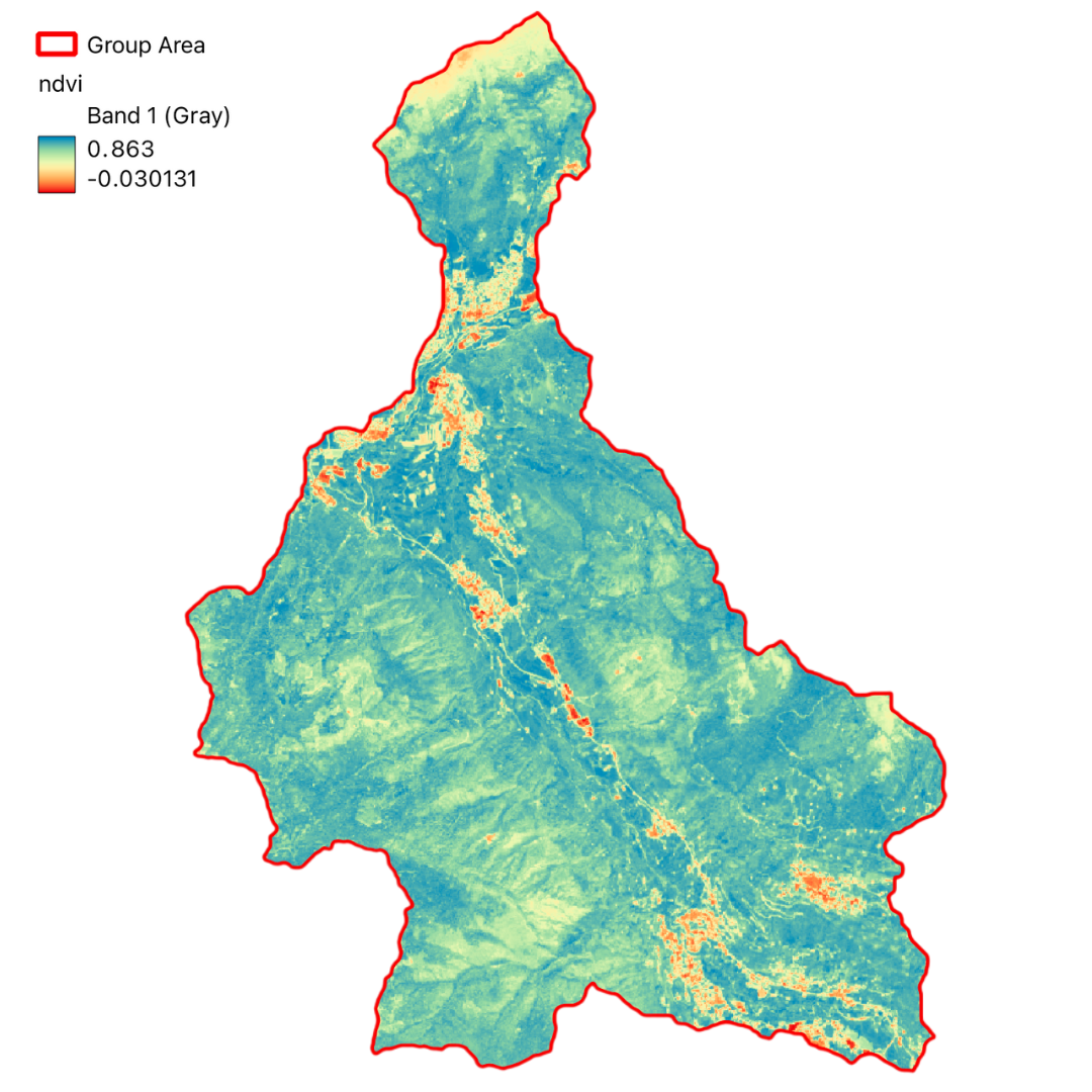
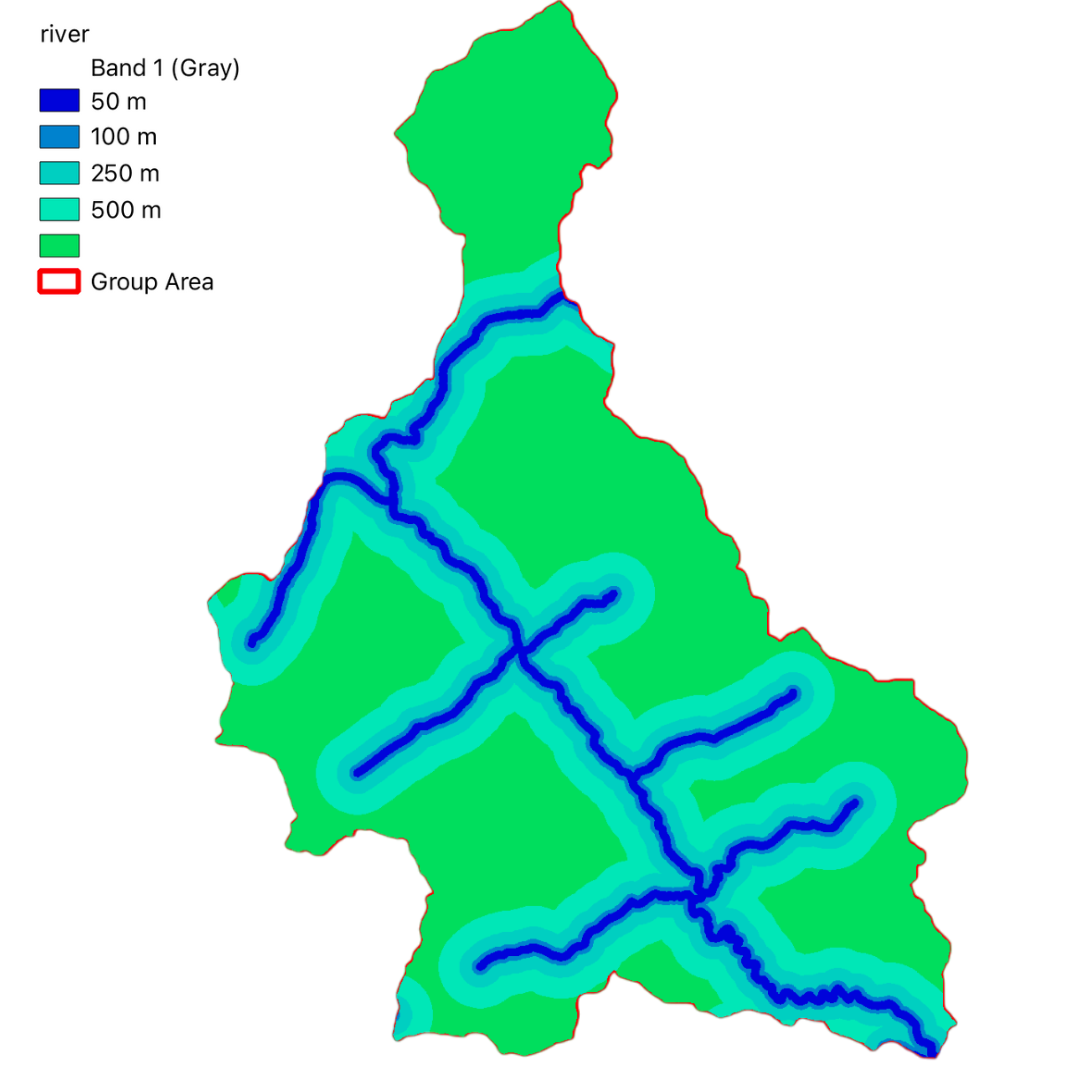
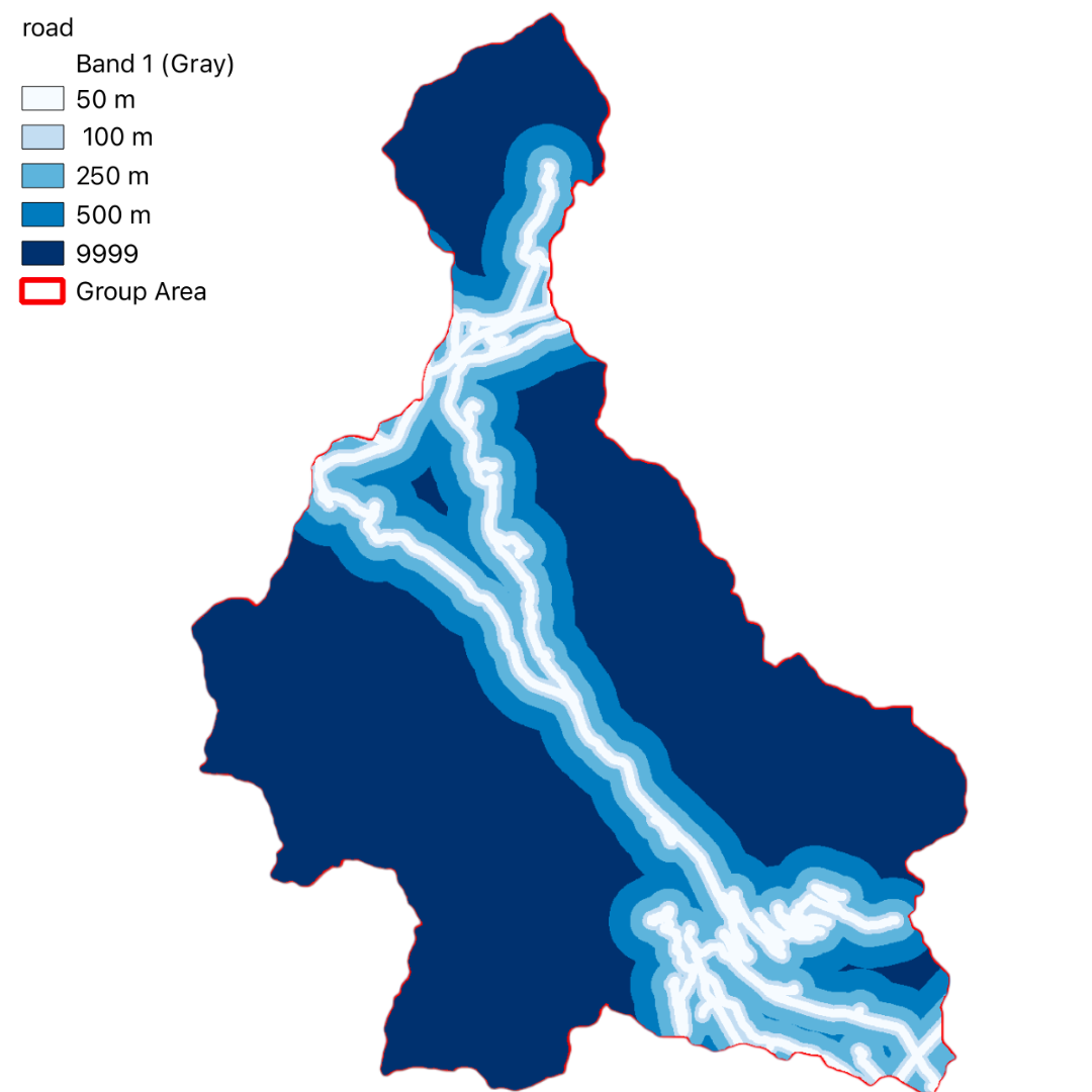
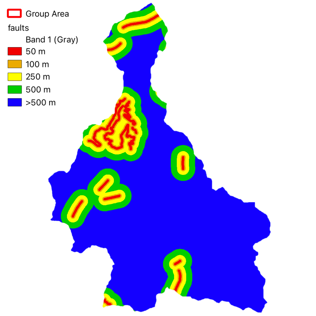
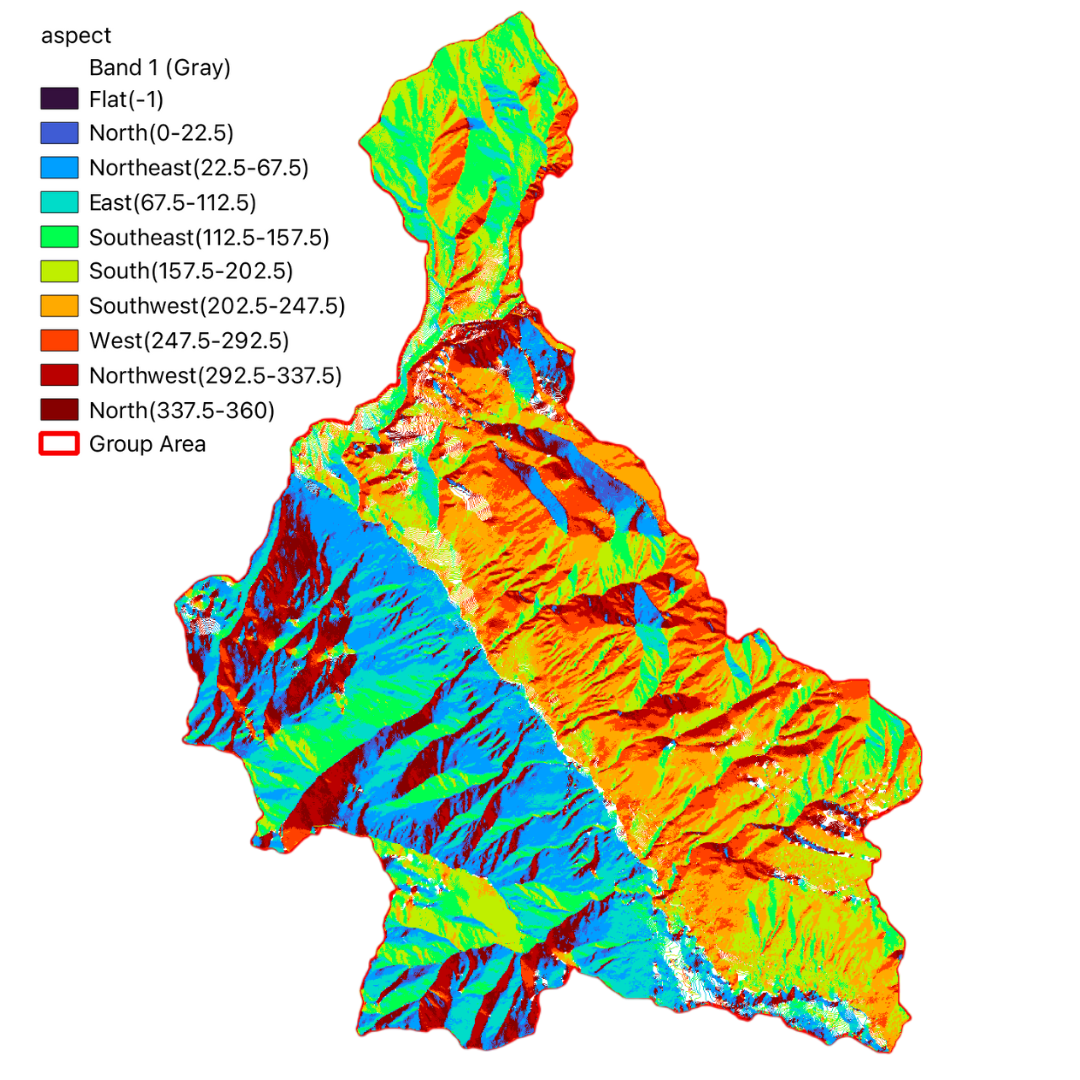
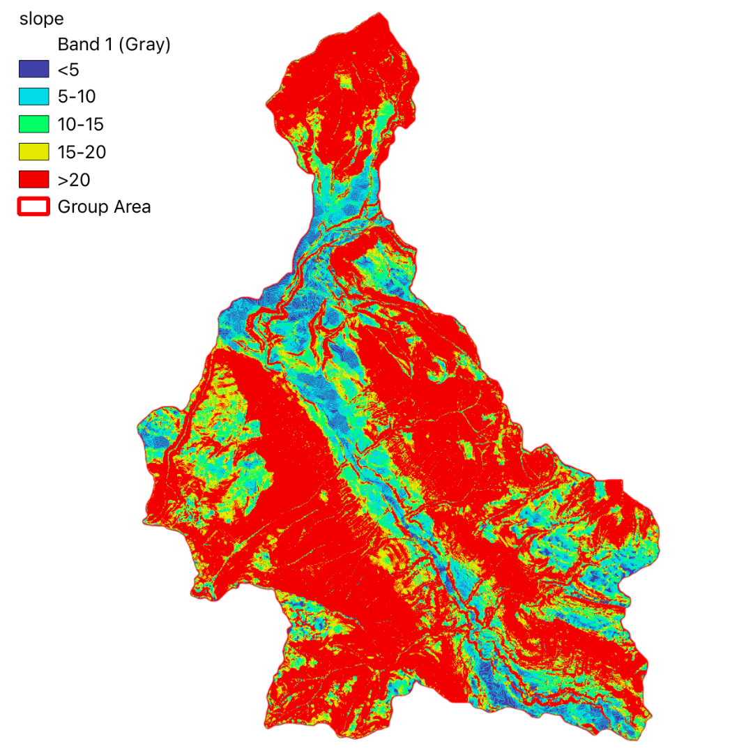
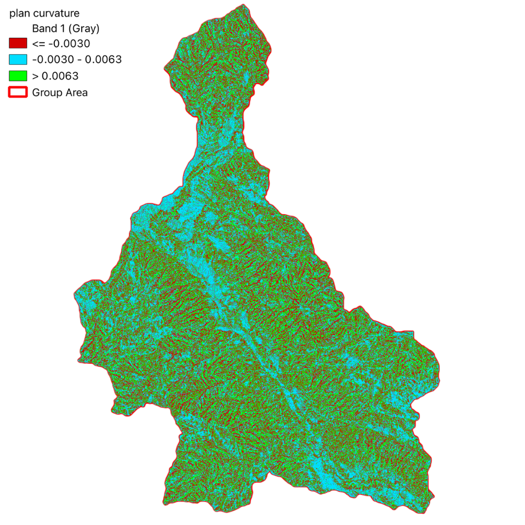
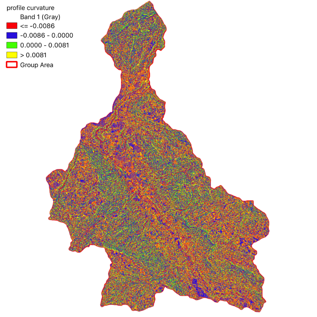
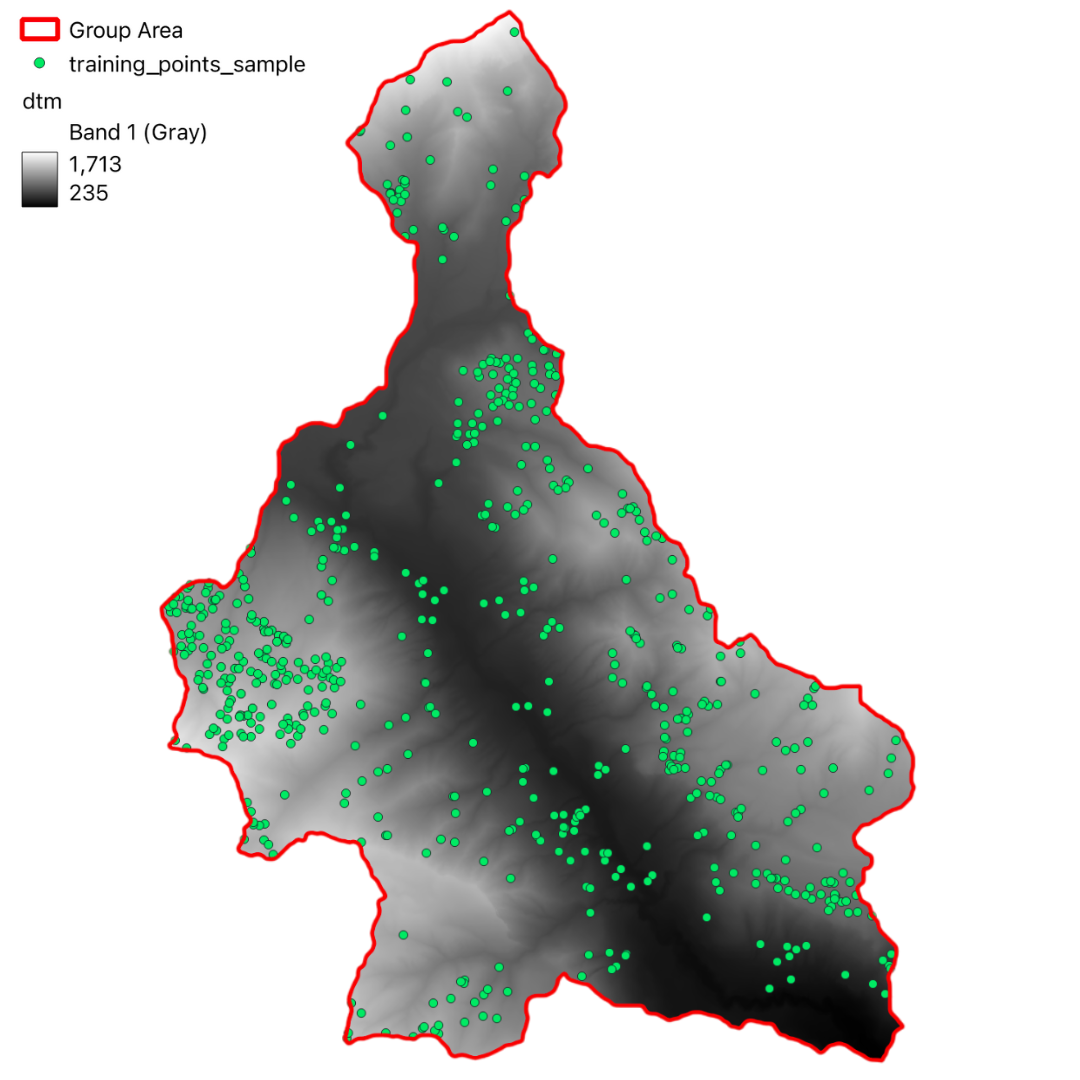
In this project, we have utilized GIS and remote sensing to integrate various datasets such as Digital Terrain Model (DTM), land use data (DUSAF), river and road buffers, landslide inventory maps, and Normalized Difference Vegetation Index (NDVI). These datasets help in understanding the terrain, land cover, proximity to water bodies and infrastructure, historical landslide events, and vegetation health, respectively.
Importance of Monitoring and Predicting Landslides
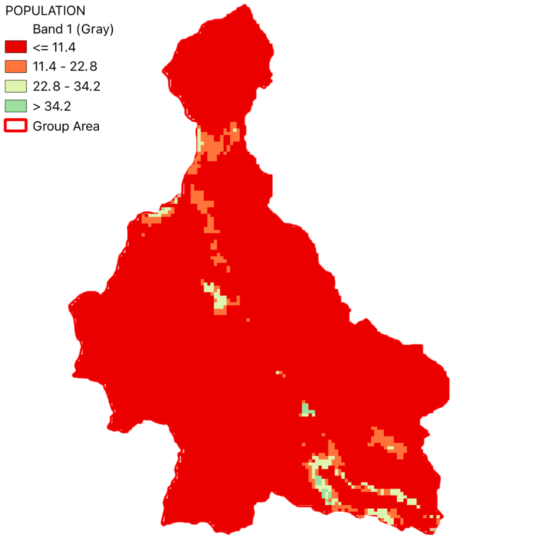
Monitoring and predicting landslides is crucial for disaster risk reduction. By identifying areas that are susceptible to landslides, authorities can implement preventive measures, plan land use more effectively, and respond promptly to potential landslide events. Evaluating the exposure of populations in these areas helps in prioritizing resources and efforts for evacuation and emergency response, thereby minimizing the impact on communities.
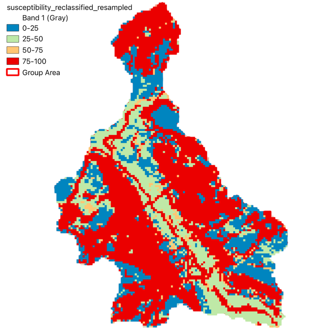
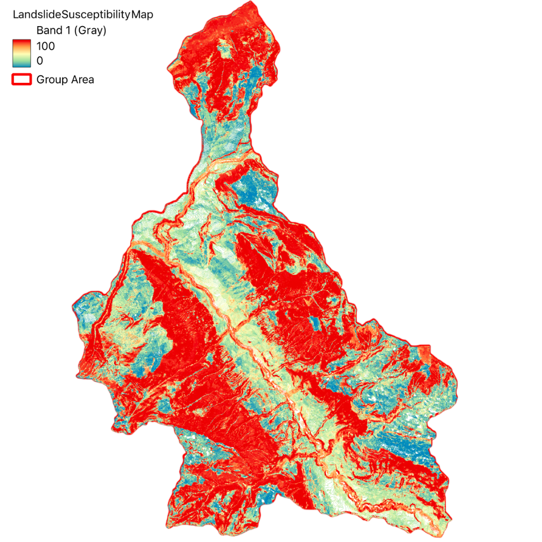
Through this project, we aim to identify areas susceptible to landslides and evaluate the exposure of the population within these areas. By integrating various datasets and utilizing advanced geospatial analysis techniques, we have generated a comprehensive landslide susceptibility map.
The final output includes a WebGIS application that provides an interactive platform for exploring the susceptibility map and related data layers. This tool not only aids in understanding the spatial distribution of landslide risk but also serves as a valuable resource for decision-makers in land use planning and disaster management.

Study Area
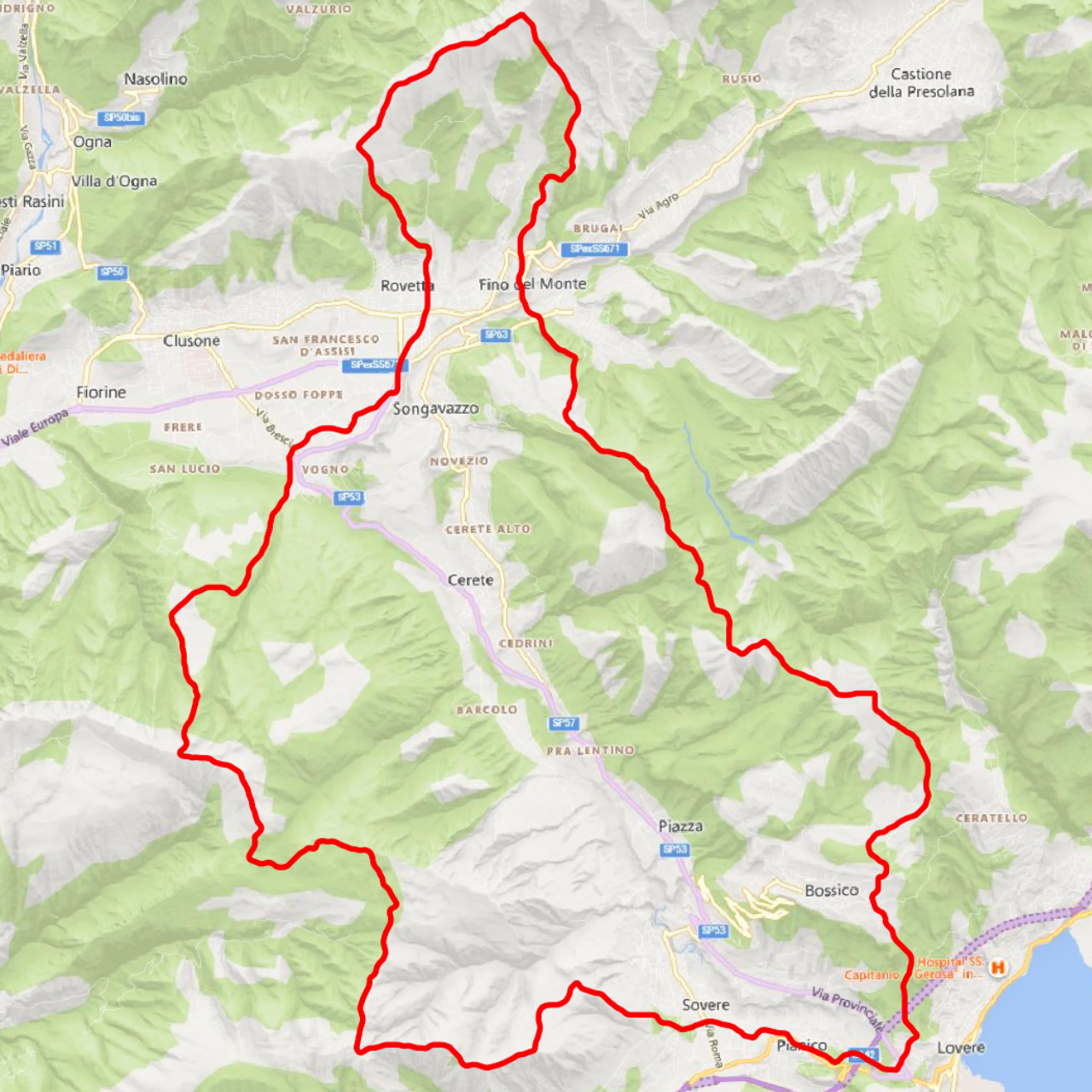
The study area is situated in the Lombardy region, within the province of Bergamo, Italy. Positioned to the north of Lake Iseo, this region encompasses an area of approximately 56 square kilometers and hosts a population of 12,109 residents. The area includes the towns of Cerete, Songavazzo, Fino del Monte, and portions of Rovetta and Sovere.
Geographic Coordinates and Extent
- Latitude: 45.85° N to 45.95° N
- Longitude: 9.85° E to 10.05° E
The study area is characterized by its diverse topography, which includes the foothills of the Alps, rolling hills, and proximity to Lake Iseo. This geographical diversity contributes to the unique environmental and climatic conditions observed within the region.
Key Urban Areas
Cerete
Coordinates 45.8801° N, 10.0567° E. Known for its historical architecture and community-oriented environment.
Songavazzo
Coordinates 45.8854° N, 9.9953° E. Noted for its scenic landscapes and outdoor recreational opportunities.
Fino del Monte
Coordinates 45.8815° N, 9.9964° E. Recognized for its tranquil atmosphere and picturesque views.
Rovetta
Coordinates 45.8920° N, 10.0512° E. A town with a rich historical heritage and natural beauty.
Sovere
Coordinates 45.8103° N, 10.0569° E. Known for its historical landmarks and scenic surroundings.
Demographic and Socioeconomic Profile
The population density of the study area is approximately 216 inhabitants per square kilometer. The socioeconomic activities are predominantly centered around agriculture, tourism, and small-scale industries. The demographic distribution exhibits a balanced age structure with a mix of young and elderly populations.
Environmental and Climatic Features
The region experiences a temperate climate with distinct seasonal variations. The proximity to Lake Iseo influences the local microclimate, contributing to milder winters and cooler summers compared to the surrounding inland areas. The area's elevation ranges from approximately 180 meters to 1,200 meters above sea level, influencing both climate and biodiversity.
About
This project is part of the Master of Science in Geoinformatics at Politecnico di Milano. The MSc in Geoinformatics program at Polimi aims to equip students with advanced skills in geographic information systems, remote sensing, and spatial data analysis. The program emphasizes the application of geoinformatics in various fields such as environmental monitoring, urban planning, and disaster management.

Politecnico di Milano
Politecnico di Milano, founded in 1863, is one of the leading technical universities in Europe. The university is known for its high-quality education and research in engineering, architecture, and design. The Department of Civil and Environmental Engineering (DICA) at Polimi is dedicated to advancing knowledge and technologies in civil and environmental engineering through innovative research and teaching.
GIS Course
The Geographic Information Systems course for the academic year 2023-2024 covers various aspects of GIS and remote sensing technologies. The course includes practical projects such as landslide susceptibility mapping and population exposure assessment, providing hands-on experience in geospatial analysis and visualization.
Course Instructors
Project Team Members
Validation
Validate the susceptibility map using accuracy assessment and sampling
Use a Python script for accuracy assessment, comparing predicted susceptibility with actual landslide occurrences to generate an error matrix for validation results and producing an error matrix to quantify the accuracy of the susceptibility map.
from qgis.core import QgsProcessing
from qgis.core import QgsProcessingAlgorithm
from qgis.core import QgsProcessingMultiStepFeedback
from qgis.core import QgsProcessingParameterFileDestination
from qgis.core import QgsProcessingParameterFile
from qgis.core import QgsProcessingParameterVectorLayer
from qgis.core import QgsProcessingParameterRasterLayer
from qgis.core import QgsProcessingParameterField
from qgis.core import QgsProcessingParameterString
from qgis.core import QgsVectorLayer
from qgis.core import QgsProcessingParameterFeatureSink
from qgis.core import QgsProject
from qgis.core import QgsFeatureSink
import processing
import numpy as np
import random
import string
import os
import pandas as pd
class Accuracy_assessment_and_sampling(QgsProcessingAlgorithm):
def initAlgorithm(self, config=None):
	self.addParameter(QgsProcessingParameterVectorLayer('vectorwithclassificationandreference', 'Vector with reference data', types=[QgsProcessing.TypeVector], defaultValue=None))
	#self.addParameter(QgsProcessingParameterVectorLayer('vectorwithclassificationandreference', 'Vector with classification', types=[QgsProcessing.TypeVector], defaultValue='C:/Users/Gorica/Documents/Teaching_2020_2021/Lab/Sampling points/stratified_random_sampling1_classified.gpkg'))
	self.addParameter(QgsProcessingParameterField('reference', 'Reference data column', type=QgsProcessingParameterField.Numeric, parentLayerParameterName='vectorwithclassificationandreference', allowMultiple=False, defaultValue=None))
	self.addParameter(QgsProcessingParameterString('Newfieldname', 'Name of new field for raster values', multiLine=False, defaultValue='Thematic_class'))
	self.addParameter(QgsProcessingParameterRasterLayer('raster', 'Raster to be sampled', defaultValue=None))
	self.addParameter(QgsProcessingParameterFileDestination('Outputfolder', 'Error matrix output path', fileFilter='CSV Files (*.csv)', defaultValue=None))
	self.addParameter(QgsProcessingParameterFeatureSink('Sampled', 'Sampled', type=QgsProcessing.TypeVectorAnyGeometry, createByDefault=True))#, defaultValue=None))
	#self.addParameter(QgsProcessingParameterVectorDestination('Sampled', 'Sampled', type=QgsProcessing.TypeVectorPoint, defaultValue=None, optional=True))

def processAlgorithm(self, parameters, context, model_feedback):
	# Use a multi-step feedback, so that individual child algorithm progress reports are adjusted for the
	# overall progress through the model
	feedback = QgsProcessingMultiStepFeedback(1, model_feedback)
	results = {}
	outputs = {}

	#reference=parameters['reference']
	#classification=parameters['Newfieldname']
	#output_folder=parameters['Outputfolder']

	# Sample raster values
	alg_params = {
		'COLUMN_PREFIX': parameters['Newfieldname'],
		'INPUT': parameters['vectorwithclassificationandreference'],
		'RASTERCOPY': parameters['raster'],
		'OUTPUT': parameters['Sampled']
	}

	SampleRasterValues= processing.run('qgis:rastersampling', alg_params, context=context, feedback=feedback, is_child_algorithm=True)


	vlayer = QgsVectorLayer(SampleRasterValues['OUTPUT'])


	idx_1 = vlayer.fields().indexFromName(parameters['reference'])
	idx_2 = vlayer.fields().indexFromName(parameters['Newfieldname'])


	list_class = []
	list_ref = []

	features =  vlayer.getFeatures()

	for ft in features:
		if ft.attributes()[idx_2]!=None and ft.attributes()[idx_1]!=None:
			list_class.append(ft.attributes()[idx_2])
			list_ref.append(ft.attributes()[idx_1])

	feedback.pushInfo(str(idx_2))
	error_matrix1=pd.crosstab(pd.Series(list_class, name=parameters['Newfieldname']),pd.Series(list_ref, name=parameters['reference']), dropna=False)

	cls_cat=error_matrix1.index.values

	#extract all columns values (classes of existing dataset)
	ref_cat=error_matrix1.columns.values
	#make union of index and column values
	cats=(list(set(ref_cat) | set(cls_cat)))
	#reindex error matrix so that it has missing columns and fill the emtpy cells with 0.00000001
	error_matrix=error_matrix1.reindex(index=cats, columns=cats, fill_value=0.00000001)
	error_matrix.index.name=error_matrix.index.name+"/"+error_matrix.columns.name

	# OUTPUT
	diag_elem=np.diagonal(np.matrix(error_matrix))
	UA=(diag_elem/error_matrix.sum(axis=1))*(diag_elem>0.01)
	PA=diag_elem/error_matrix.sum(axis=0)*(diag_elem>0.01)
	OA=sum(diag_elem)/error_matrix.sum(axis=1).sum()
	error_matrix['UA']=UA.round(2)
	error_matrix['PA']=PA.round(2)
	error_matrix['OA']=np.nan
	error_matrix.loc[error_matrix.index[0],'OA']=OA

	error_matrix.to_csv(parameters['Outputfolder'])
	feedback.pushConsoleInfo('Error matrix saved in '+parameters['Outputfolder'])
	return results

def name(self):
	return 'Accuracy_assessment_and_sampling'

def displayName(self):
	return 'Accuracy assessment and sampling'

def group(self):
	return 'raster'

def groupId(self):
	return ''
def createInstance(self):
	return Accuracy_assessment_and_sampling()
Algorithm Description
This algorithm takes sample points with reference classes and sample raster in the same location of sample points. Then it estimates error matrix and accuracy indexes by cross tabulating field with reference classes and field with classification classes.
Input Parameters
- Vector with Reference Data: Vector of sampling points which are already classified (i.e. reference point data).
- Raster to be Sampled: Raster is the thematic map for which accuracy is being estimated. This raster will be sampled in the location of sampling points.
- Reference Data Column: Name of the column in which sampled raster values will be stored.
Outputs
- Error Matrix Output Path: Mandatory!!! Path and name of the output file with error matrix and accuracy indexes. Accuracy indexes estimated are Overall accuracy, User's accuracy, and Producer's accuracy.
- Sampled: Mandatory!!! Path and name of the output vector file that contains all the data as "Vector with reference data" plus the new column with values sampled from raster.
Algorithm Author: Gorica Bratic
Algorithm Version: 1.0
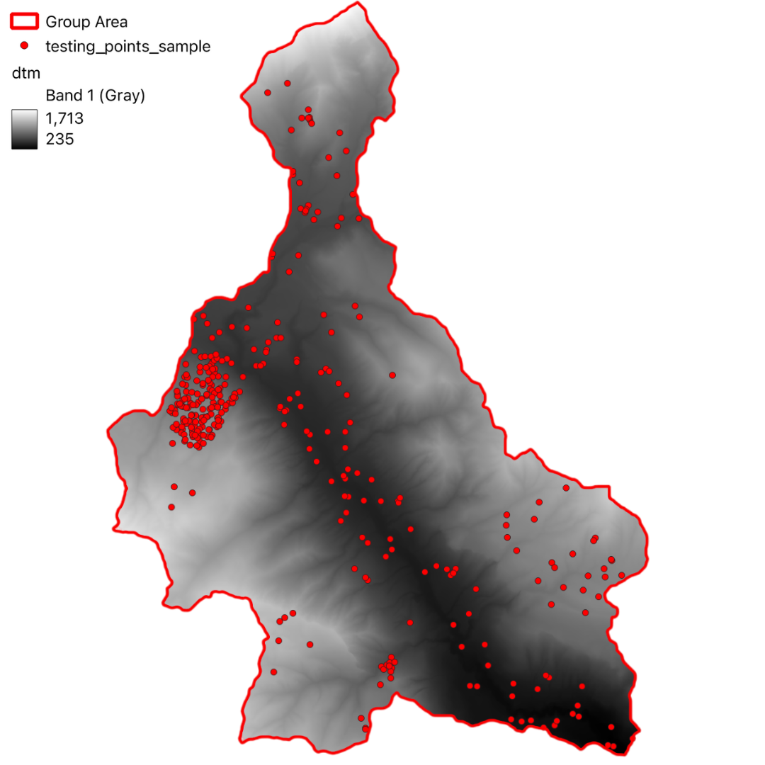
Testing Points
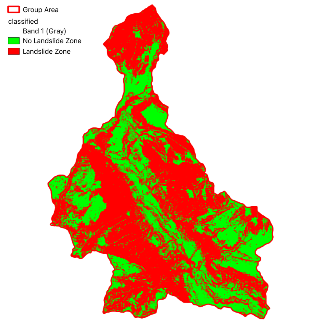
Classification
Error Matrix and Validation
To validate the accuracy of our susceptibility map, we computed an Error Matrix using a subset of known landslide locations. The following table presents the computed matrix:
| Predicted/Actual |
No Landslide |
Landslide |
UA |
PA |
OA |
| No Landslide |
120 |
77 |
0.61 |
0.80 |
0.69 |
| Landslide |
30 |
118 |
0.80 |
0.61 |
|